Overview
Sparklines is a fast and very convenient tool for analysis the dynamics of any data ranges. If you need to quickly analyze a large number ranges of different indicators and surprise your boss with how little you spent your time on it – the Sparklines is a tool you must know.
Creating Sparklines
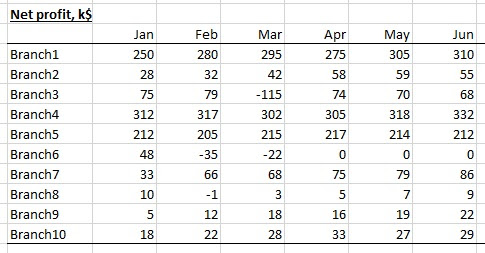
For example, you have some data ranges you have to analyze:
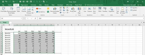
- Select a range of cells you want to analyze.
- Click “Insert” on the main menu.
- Click “Line”, “Column” or “Win/Loss” on the “Sparklines” sector.
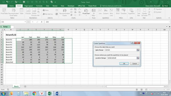
Changing parameters of Sparklines
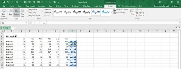
- Choose any sparkline.
- Click “Design”.
- You can change the type of sparkline in “Type” sector.
- You can highlight different elements of sparklines in the “Show” sector.
- You can change style of sparklines in the “Style” sector.
- You can change the data range in “Sparkline”sector.
- You can change Axis parameters, ungroup sparklines, delete sparklines in the “Group” sector.
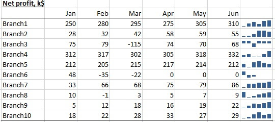
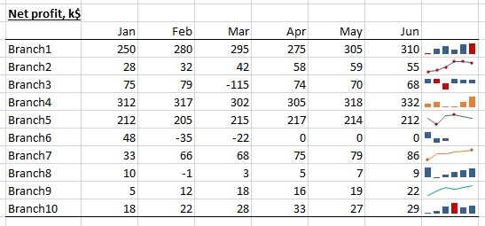
After changing sparklines parameters, you can see something like this:
Conclusion
This excel feature is a cool tool to impress your boss. With Sparklines you can show how fast and easily you can analyze a large number of different indicators. With Sparklines you can easily create a lot of little charts and highlight important things.
If you have any questions with respect to Excel , please reply to this email, we will quickly give you solution to your Excel Problem.
